Hello All!
There were some questions on the first day of class regarding my example of 2 researchers A(lice) and B(ob), and how to interpret their p-values. To refresh your memory, the example is here:
I made a simplifying assumption I’d like to clarify, and discuss the basic idea here with some pictures to help explain. Hopefully this post fill any holes in this example; I went through it at a pretty brisk pace.
A Brief Review
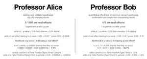
We have different priors about Professors Alice and Bob– Alice is looking for less-likely but more-important effects to see if they’re real, and (like looking for a needle in the haystack) we’d expect her to test a real effect only rarely (1 out of 1000 tests). Bob is taking a more conservative approach, and is simply quantifying the effect sizes of things we all are already pretty sure are true (things like candy causes cavities… but how big is the effect?). He happens to test real effects 4 times out of 5 because of this strategy.
We can see from the math above that a p value less than 0.05 means very different things for these two professors. For Alice, an occurrence of p<0.05 has only a 1.8% chance of being caused by a real underlying effect rather than random sampling noise; for Bob, that same p<0.05 is over 98% likely to be suggestive of a real effect.
A p-value for Bob of p<0.05 is much, much more trustworthy than a p-value for Alice at p<0.05. It is indicative of a real underlying effect 98% of the time vs a measly 1.8%.
I made this point in lecture, and want to reiterate it here. If you have a negative reaction to this statement about interpreting Bob’s and Alice’s p-values at p<0.05– as though I’ve made a value judgement that Bob’s research is good and Alice’s is bad— it means you’ve deeply internalized a categorical and deeply flawed worldview of p-values. Saying that a p-value for Bob of p<0.05 is more trustworthy than Alice at p<0.05 is not a value judgement of them as researchers; it’s a statement about whether applying alpha=0.05 is meaningful when trying to interpret their work.
I think most of us (myself included) would rather be Alice in this example; she is researching unintuitive, surprising, and paradigm shifting hypotheses. She is a good and trustworthy researcher– they’re both running studies at 90% power in this example. The point is that the p-value means something very different for each of them, and should be interpreted very differently for each of them. Using an alpha of 0.05 to judge Alice, given our intuition, is simply silly. That’s not a judgement of Alice’s work; it’s a statement about how we should contextualize it. We should revise down this alpha value for Alice based on our priors, until we believe the evidence actually supports the existence an underlying effect; this reasoning process is completely dependent on our intuition. When you’re uncertain, err on the side of caution.
The odds that data surpassing our alpha threshold provides evidence of an underlying effect is called the PPV. It is not the same as a p-value, even though many people conflate the two. If you’ve made this mistake, you’re not alone; over 80 percent of statistics teachers and 40% of psychology teachers make some form of it. The above example shows us how to think about PPV given a p-value; we need to be doing this calculation in our heads whenever we interpret a p-value.
Clarifications
There was some confusion about the math on that slide, so I want to walk through it in detail. I find, when thinking about probability, it’s often easiest to think graphically about what we’re calculating:
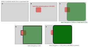
So let’s say (A) that we draw out of world of possible experiments as a grey box. We’ll be working in percentages, so it’s easy to think of this as grey box as representing 100 experiments that Professor Bob is running. Now we know that (B) alpha is 0.05, which means there is a 5% chance of getting a false positive if none of our experiments have real effects. In other words, if we ran 100 experiments, we’d expect 5 of them to have a p-value < 0.05 just from sampling noise (that’s the definition of a p-value). These 5% of test results are represented in red.
Now we’ll highlight the tests that give a p-value<0.05 due to a real effect in (C). From Bob’s example, we’ve said 4 of every 5 tests Bob runs has a real effect, and Bob is running his tests at 90% power (what a great researcher!). Since power tells us the likelihood of a value below our alpha cutoff (of 0.05) if a real effect is present, the odds of p<0.05 due to a real effect is equal to 4/5 * 0.9 in this case, or 72 out of 100 tests. So when Bob runs 100 tests, 80 of them have a real effect, and we expect to correctly catch 72 of those with a p<0.05 because Bob is such a good researcher and does his experiments with a high, 90% average power.
Notice that these real effects overlap with the 5 tests where we expect random noise. In other words, these events are independent.
Initially we said that we would expect 5 out of 100 tests to give us a p-value < 0.05 from noise; If we look at the subset of tests left over after we account for the ones we labeled in green, we’d still expect 5% of these to give us a p-value < 0.05 because of noise (5% of our 28 leftover tests in the section outside of the green, or roughly 1 test in our example). That one test is represented in the non-overlapping red section.
We can think about calculating the non-overlapping red area in two equivalent ways. We just described an intuitive way– 5% of the grey area left outside of the green. The grey leftover is 100%-72%=28%. We could calculate this non-overlapping red area then as five percent of it, or 0.28*0.05 = 1.4%.
We could also subtract the overlapping red-green area from the overall red area. Because the red and green events are independent, we know that the overlapping area represents 72% of the red area, just as the green represents 72% of the grey. In this case we can simply calculate it as 0.05 – 0.05*0.72 = 1.4%.
Notice that in this example, the overlapping section starts to lose meaning, because it represents contradictory assumptions. That section represents the percentage of the 72 tests– tests that have a p-value < 0.05 because of a real effect– that otherwise would’ve had a p-value < 0.05 from noise if there *wasn’t* a real effect. That assumption is now invalid. What we have left to really work with is the red and green areas by themselves.
So this is the world we live in. We have 72 tests in green that have a p<0.05 effect due to a real underlying effect, and we have the non-overlapping part of the red section that represents the number of tests giving us a p<0.05 values due to noise, which we found to be 1.4 tests out of 100.
Now we want to know a conditional quantity– what is the likelihood of a real effect given we see p<0.05? In other words, what percentage of the area represented in (D) does (E) represent?
This makes our final calculation easy; if we want to know what the odds are that a ‘significant result’ of p<0.05 represents an actual underlying phenomena, we can simply take the fraction of the green+red area consumed by the green alone.
As we saw in our initial example, for a researcher with an 80% prior and 90% power, that tells us that conditioned on a test returning p<0.05, ~98% of those results will represent true underlying effects. For a more adventurous researcher tackling more unusual and unlikely hypotheses however (0.1% prior with the same 90% power), this p<0.05 category only represents a true effect 1.8% of the time.
What’s wrong with this example?
I believe the above example is a useful one to help think through when you’re looking at a p-value. You have some concept of your prior; how big is the green area (power * prior)? How much red is left in our alpha when we remove a (power * prior) fraction? What is their ratio? I encourage you to try and imagine the size of these squares for Alice and see if you can reason about the likelihood that a p<0.05 is meaningful for her, since our pictorial example is with Bob.
However, while the above construction is a good heuristic, it includes a simplification that we should fix if we want to be precise. See if you can identify it before we move on.
Here’s the answer: we left tests with a real underlying effect that fail to return a ‘significant’ p<0.05 unaccounted for. I’ve added these tests back in below.
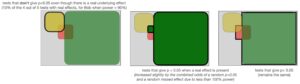
In our Bob example, we’re talking about the the 8 tests of out the 28 falling outside of the green area that still have real underlying effects we didn’t catch because our test wasn’t powerful enough. Remember, because we assumed a study power of 90%, we only caught 72 of the 80 real effects! Thus, the area of non-overlapping red that represents a p-value of random chance (5% * 28% = 1.4%) still has an 8/28 = ~29% chance of representing a real effect from pure chance.
In other words, there is a small chance that (a) we have a real effect, (b) our test didn’t catch it with p<0.05 because our study power isn’t a perfect 100%, AND (c) we happen to get ‘lucky’ and hit a p<0.05 simply from from noise where we otherwise would’ve missed the real effect. When this rare combination happens, we still have a ‘true positive’.
Once again, in our Bob example, that means we actually have an additional 8/28 = 29% chance, multiplied by the non-overlapping red section (1.4%), to get a ‘true positive’. 0.014*(.08/.28) gives us an additional 0.004 true positives (0.4 out of 100 tests). Notice that the overall odds of a p-value < 0.05 didn’t changed.
That means our 98.1% confidence in a p-value < 0.05 for Bob should actually be revised up slightly to 98.6%
(0.72 + 0.004) / (0.72 + (0.05-0.036)) = 98.6%
Our example for Alice can also be corrected, though this correction doesn’t change the result because it’s so so small, just 0.000005:
(.05-0.000045) * ((0.001 – 0.001*0.9)/(1- 0.001*0.9)) = 0.000005
(0.0009 + 0.000005) / (0.0009 + (0.05-0.000045)) = 1.8%
Most of the time (if we’re doing a quick gut-check), this quantity shouldn’t matter much. Intuitively, we need to worry about this correction when we have a low power and a large prior. That’s the only time we’ll get a significant percentage of the area outside of the true effect, p<0.05 area that still represents real effects.
A low power and a large prior don’t typically go together; to practically achieve this we’d have to test something very certainly true, but with a small effect size and sample size.
This correction represented in color on a contour plot (percentage) plotted as a function of the prior (x) and the experimental power (y). [z = (x-x*y)/(1-x*y), x=[0,1], y=[0,1]] Again, this is the fraction of non-significant results that are ‘incorrect’, i.e. a real effect is present but we failed to reject the null hypothesis. The correction grows as we increase the prior (x) and decrease the power (y).
When we have an 100% prior (every experiment has a real underlying effect), every non-significant finding is a ‘false negative’ and we need to ‘correct’ 100%. When we have a 0% prior (we tested no real effects), every non-significant finding is, in fact, a non-result, so we need 0% correction.
A note on PPV calculations
What we’ve just done is called a PPV calculation, and I hope this explanation felt approachable and built some of your intuition. Remember that PPV is the thing we care about– how likely an effect is to be real given a p-value below alpha.
With our intuition cemented, the caveats we introduced as we moved towards analytical precision start to turn a mental check into something that feels hard to calculate. Luckily, the math actually simplifies to a very tidy equation, which is described in detail in Power Failure: why small sample size undermines the reliability of neuroscience:
PPV = power*R / (power*R + alpha).
The definition for R is a slightly confusing one— instead of a prior probability, we use a simple pre-study odds ratio.
Try it out and be amazed! In our example above, R is 4/1 for Bob and 1/999 for Alice. When we plug these ratios in with our power (0.9 for both) and our alpha (0.5), you’ll see we get exactly the numbers we arrived at in our example with a lot less work: 98.6% and 1.8%.